Ecosystems and Biogeochemical Models
The Terrestrial Ecosystem Model
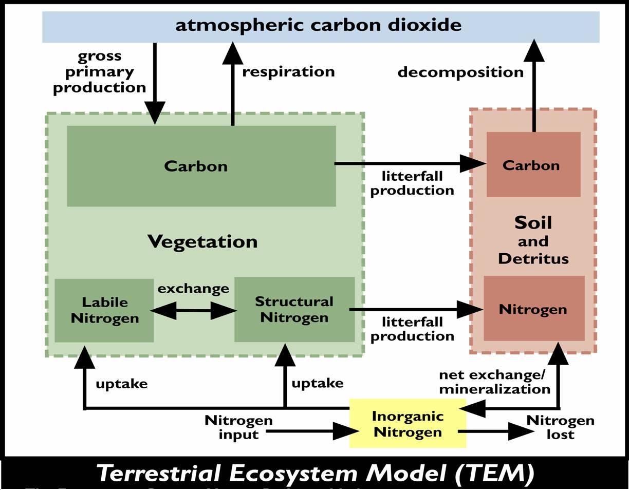
The Terrestrial Ecosystem Model (TEM) is a process-based ecosystem model that describes carbon and nitrogen dynamics of plants and soils for terrestrial ecosystems. The TEM uses spatially referenced information on climate, elevation, soils, vegetation and water availability as well as soil- and vegetation-specific parameters to make monthly estimates of important carbon and nitrogen fluxes and pool sizes of terrestrial ecosystems. The TEM now operates on global scale, at a monthly time step and a 0.5 degrees latitude/longitude spatial resolution.
Following is a structure diagram of TEM:
Soil thermal model (STM)
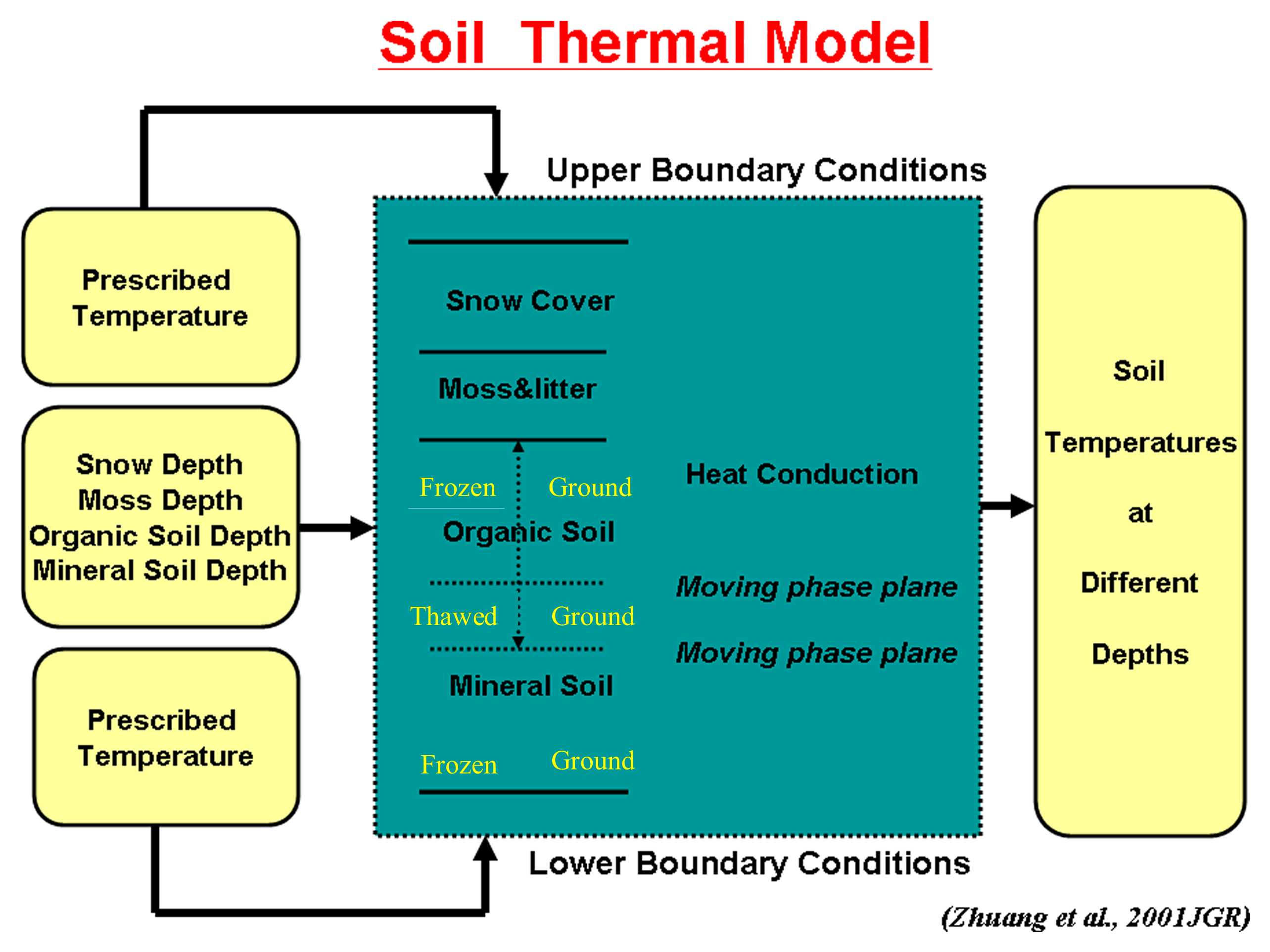
The STM was developed based on the Goodrich model, the vertical profile is divided into snow cover, moss, upper organic soil, lower organic soil, and mineral soil layers (Figure 1a). Appli-cation of the model for a site requires specification of the thickness of each layer and simulation depth steps within each layer. The thermal properties of each layer also need to be prescribed. In addition, the dynamics of phase changes in the soils depend on the phase temperature, which we set to 0oC for applications of the model in this study. Specification of the upper boundary condition includes the temperature at the top of the moss layer during the summer and at the surface of snow during the winter. In this study we prescribed the depth, density, and thermal properties of snow cover. For the lower boundary condition we assumed a constant heat flux. Alter-natively, the lower boundary condition can be specified as a temporally varying function of temperature or heat flux. Ap-plication of the model requires the prescription of initial con-ditions, which include specifying the initial soil temperatures of the system and the presence or absence of permafrost (Zhuang et al., 2001).
Following is a diagram of the STM:
Water Balance Model 1.0
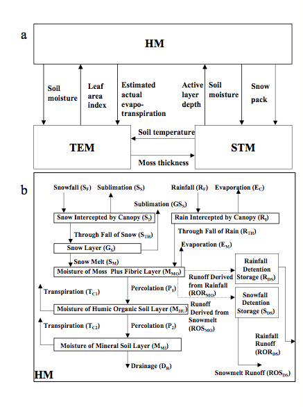
Fig.1 Sturcture diagram for Water Blance Model 1.0
Fig. 1. (a) Overview of the model used in this study, which required coupling a hydrological model (HM) with a soil thermal model (STM) and a terrestrial ecosystem model (TEM). The HM receives information on active layer depth from the STM and information on leaf area index from TEM. The STM receives information on moss thickness from TEM and information on soil moisture and snow pack from the HM. The TEM receives information on soil temperature from STM and information on soil moisture and evapotranspiration from HM. (b) The HM considers the dynamics of eight state variables for water including
- rain intercepted by the canopy (RI),
- snow intercepted by the canopy (SI),
- snow layer on the ground (GS),
- moisture content of the moss plus fibric organic layer (MMO),
- rainfall detention storage (RDS),
- snowfall detention storage (SDS),
- moisture content of the humic organic layer (MHU), and
- moisture content of the mineral soil layer (MMI).
The HM simulates changes in these state variables at monthly temporal resolution from the fluxes of water identified in Fig. 2b, which include
- Rainfall (RF),
- Snowfall (SF),
- canopy transpiration (TC = TC1 + TC2),
- canopy evaporation (EC),
- through fall of rain (RTH),
- canopy snow sublimation (SS),
- through fall of snow (STH),
- ground snow sublimation (GSS),
- soil surface evaporation (EM),
- snow melt (SM),
- percolation from moss plus fibric organic layer to humic organic layer (P1),
- percolation from humic organic layer to mineral soil layer (P2),
- runoff from the moss plus fibric layer to the rainfall detention storage pool (RORMO),
- runoff from the moss plus fibric layer to the snow melt detention storage pool (ROSMO),
- runoff from the rainfall detention storage pool to surface water networks (RORDS),
- runoff from the snow melt detention storage pool to surface water networks (ROSDS), and
- drainage from mineral soil layer to ground water (DR) (Zhuang et al., 2002)
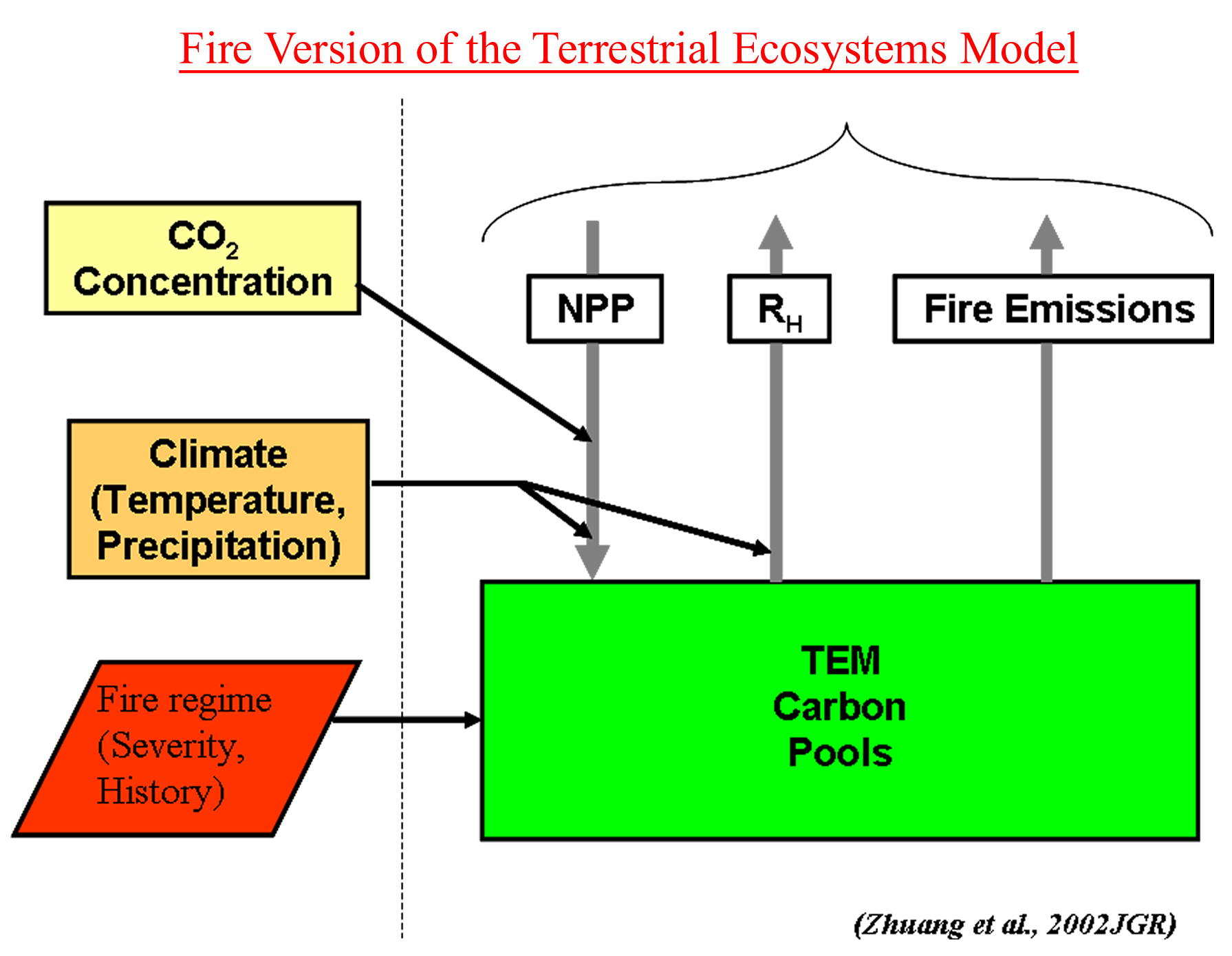
Fire version of TEM
In this version of TEM, we integrated more effective algorithms of biogeochemistry after fire with the soil thermal dynamics simulated by STM and the hydrology simulated by HM. After fire, the STM and HM require information from TEM on how the thickness of moss and leaf area index change. Therefore, we modified TEM by including formulations to simulate changes in the thickness of moss, canopy biomass, and leaf area index as the stand recovers from disturbance. The TEM requires information from STM on soil temperature and from HM on soil moisture of the humic organic layer and on estimated actual evapotranspiration (EET). We modified TEM so that soil temperature and soil moisture of the humic organic soil layer influences the simulation of heterotrophic respiration, nitrogen mineralization, and nitrogen uptake by the vegetation. Similar to previous versions of TEM, EET influences the simulation of gross primary production (GPP) (Zhuang et al, 2002).
Following is a structure diagram of the FireTEM
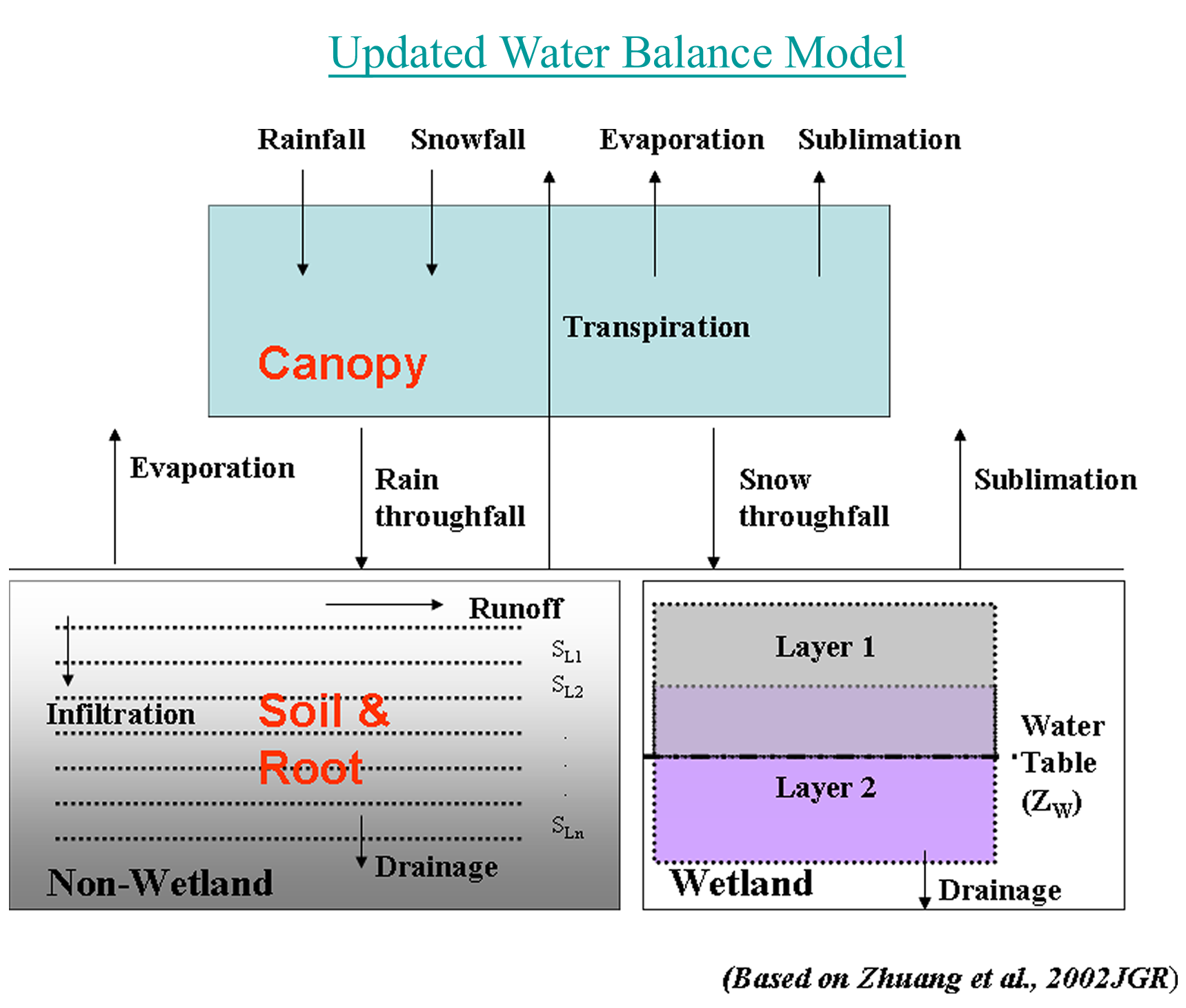
Updated Water Balance Model (WBM)
The hydrological module [HM, Zhuang et al., 2002] was further developed including:
- the consideration of surface runoff when determining infiltration rates from rain throughfall and snow melt;
- the inclusion of the effects of temperature and vapor pressure deficit on canopy water conductance when estimating evapotranspiration based on Waring and Running [1998] and Thornton [2000];
- a more detailed representation of water storage and fluxes within the soil profile of upland soils based on the use of the Richards equation in the unsaturated zone [Hillel, 1980]; and
- the development of daily estimates of soil moistures and water fluxes within the soil profile instead of monthly estimates.
As the original version of the HM is designed to simulate water dynamics only in upland soils, algorithms have also been added to simulate water dynamics in wetland soils. For wetlands, the soil profile is divided into two zones based on the water table depth: 1) an oxygenated, unsaturated zone; and 2) an anoxic, saturated zone. The soil water content and the water table depth in these wetland soils are determined using a water-balance approach that considers precipitation, runoff, drainage, snow melt, snow sublimation, and evapotranspiration. We assume that wetland soils are always saturated below 30 cm, which represents the maximum water table depth [Granberg et al., 1999]. Daily soil moisture at each 1 cm depth above the water table is modeled with a quadratic function and increases from the soil surface to the position of the water table [Granberg et al., 1999]. Infiltration, runoff, snowmelt, snow sublimation and evapotranspiration are simulated in wetlands using the same algorithms as for uplands. Drainage from wetlands is assumed to vary with soil texture, but does not exceed 20 mm day-1 (Zhuang et al., 2004GBC).
Following is a structure digram of the Updated WBM
Land-Use and Land-Change version of TEM
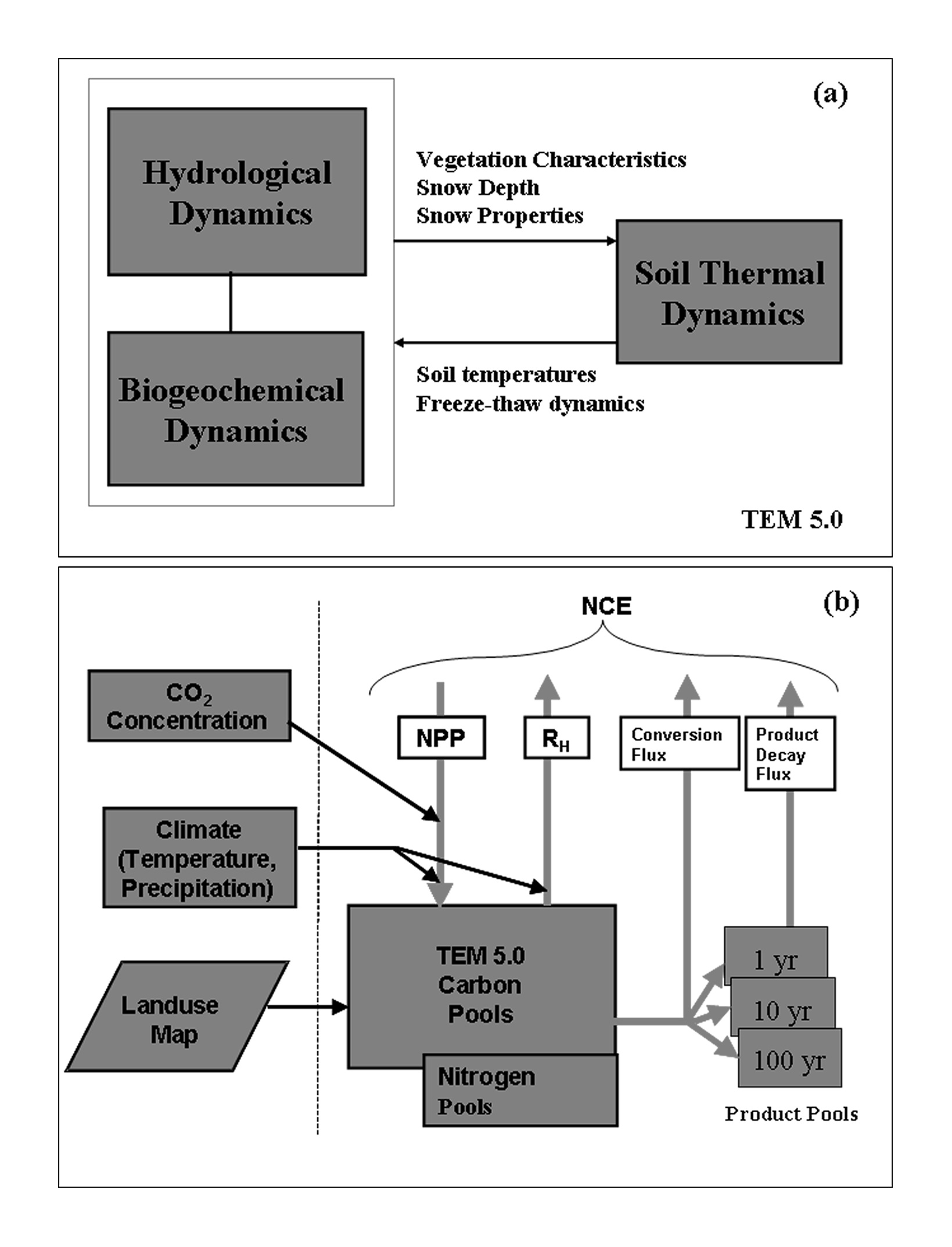
Fig.2 Structure diagram for TEM 5.0
Fig. 2. (a) The structure of TEM 5.0 includes (1) hydrological dynamics based on a Water Balance Model (WBM, Vorosmarty et al., 1989), biogeochemistry dynamics based on the Terrestrial Ecosystem Model (TEM 4.2, McGuire et al., 2001), and soil thermal dynamics based on the Soil Thermal Module (STM, Zhuang et al., 2001). Among the three components, the STM receives vegetation characteristics from TEM, receives snow depth and snow properties from the WBM, and provides simulated soil temperatures and freeze-thaw dynamics to TEM to drive ecosystem processes. (b) Overview of the simulation protocol implemented by TEM 5.0 in this study to assess the concurrent effects of increasing atmospheric CO2, climate variability, and cropland establishment and abandonment during the 20th Century.
Methane Model
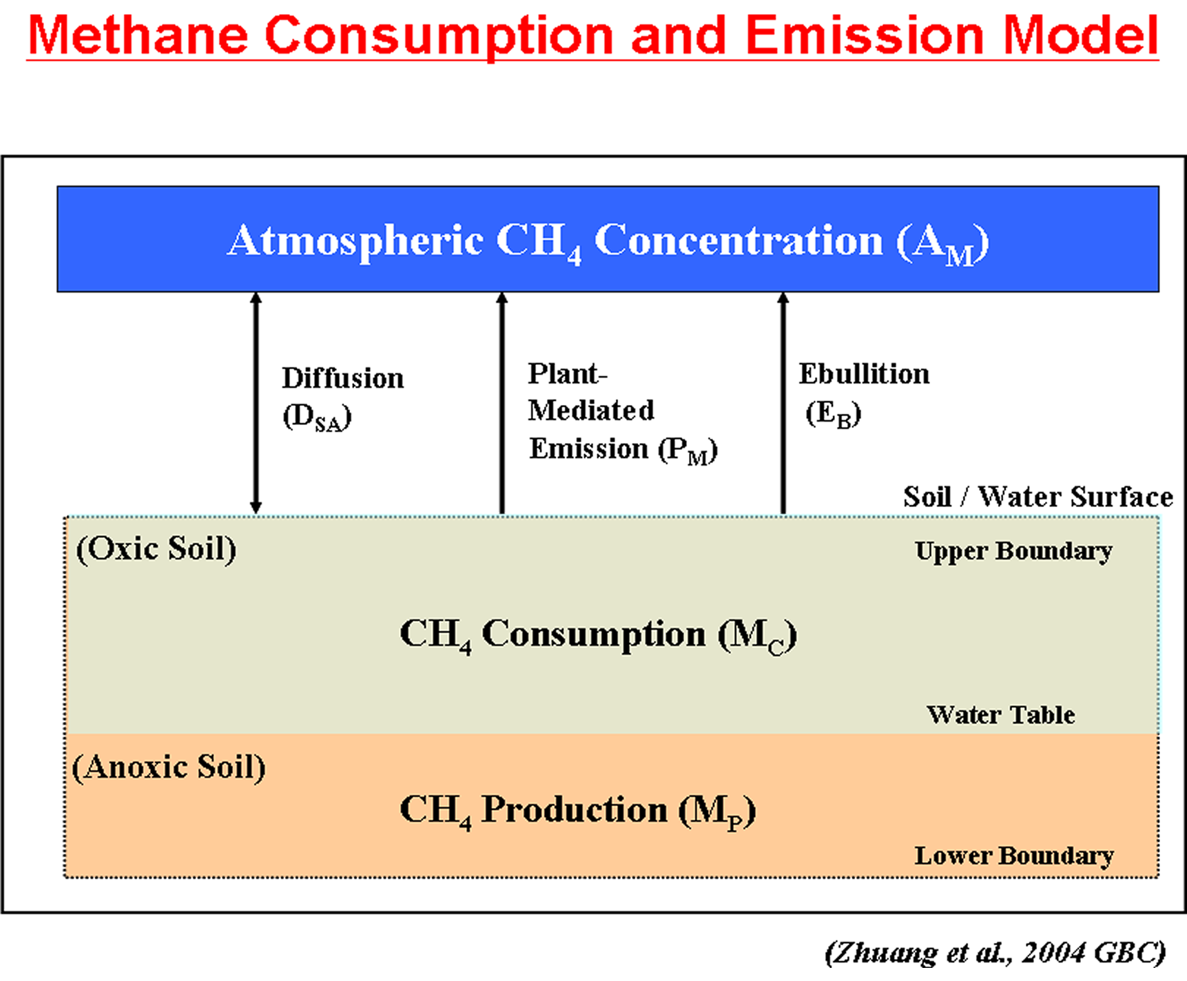
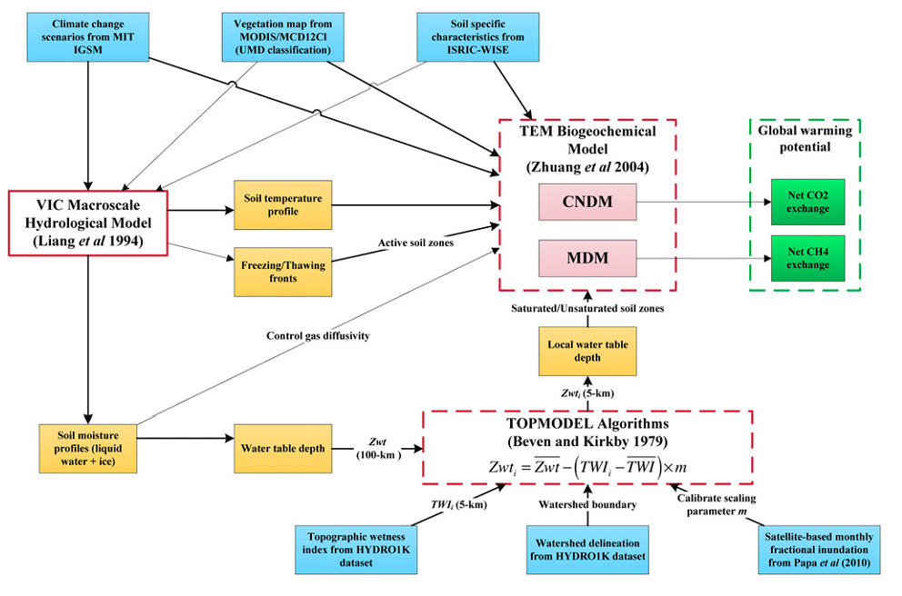
Methane Modeling Framework
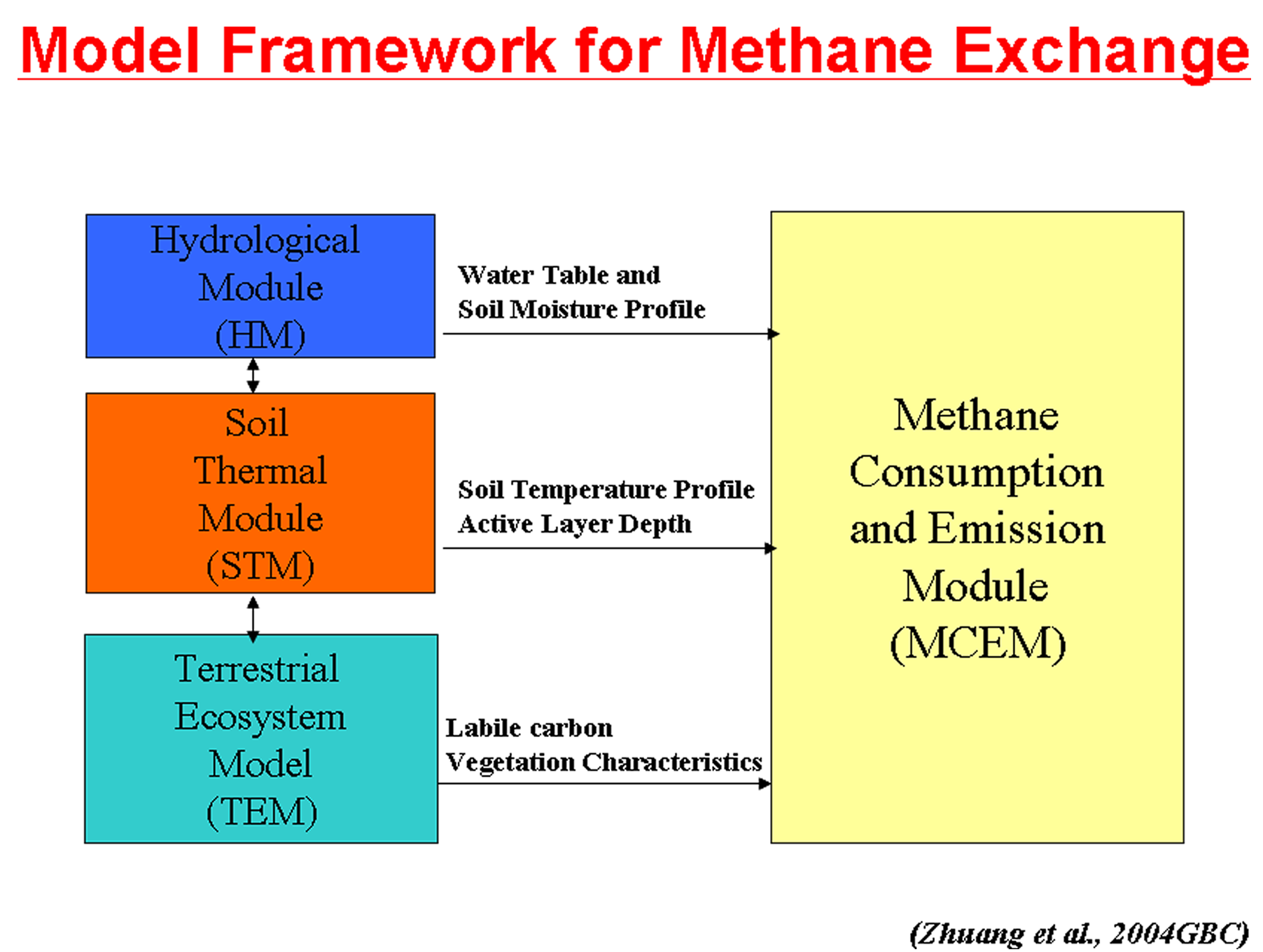
Fig. 1. Conceptual framework of coupled models to estimate net fluxes of methane and carbon dioxide. Shown are external spatial inputs (blue) for driving or calibrating models, internal information exchange (yellow) between models, and final model outputs (green). Arrows indicate the direction of information exchange among all components. See text and supplementary materials for details (available at stacks.iop.org/ERL/8/045003/mmedia) (Zhu et al., 2013).
Conceptual Framework of coupled models
N Cycling Model
Fig. 1. N cycling among the atmosphere, biosphere, and pedosphere. Major processes were modeled in AgTEM. SOM, soil organic matter; N2, nitrogen; NH3, ammonia; NOX, nitrogen oxides; N2O, nitrous oxide; NO, nitric oxide (Qin et al., 2013a).

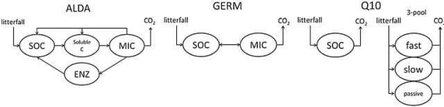
Soil Decomposition Model
Fig. 1. Uncertainty analysis of the fate of soil organic carbon with conceptually different decomposition models (He et al., 2014)
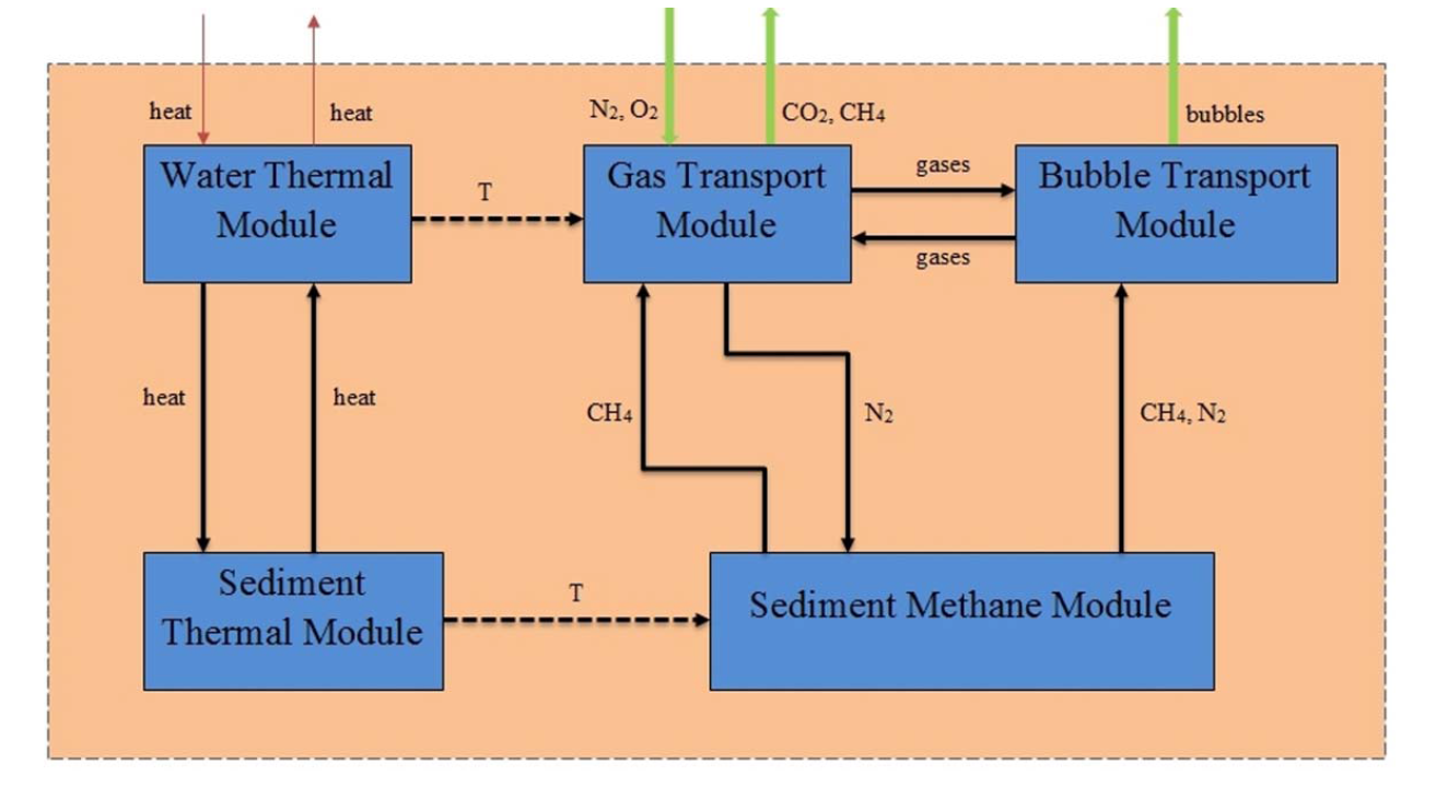
BLake4Me Model
Fig. 1. The framework of the bLake4Me model (The lake model includes a water thermal model (WTM), a sediment thermal model (STM), a gas transport model (GTM), a sediment gas model (SGM), and a bubble transport model (BTM); the solid arrow indicates energy or substance transport and the dashed arrow indicates process dependence). (Tan et al., 2015)
Peatland Model
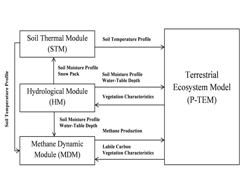
Figure 1. P-TEM modeling framework includes a soil thermal module (STM), a hydrologic module (HM) for peatland, a carbon/ nitrogen dynamic model (TEM) for peatland, and a methane dynamics module (MDM) [Wang et al., 2016a, 2016b, Zhuang et al., 2002, 2004, 2006].
3D-Hydrological Model
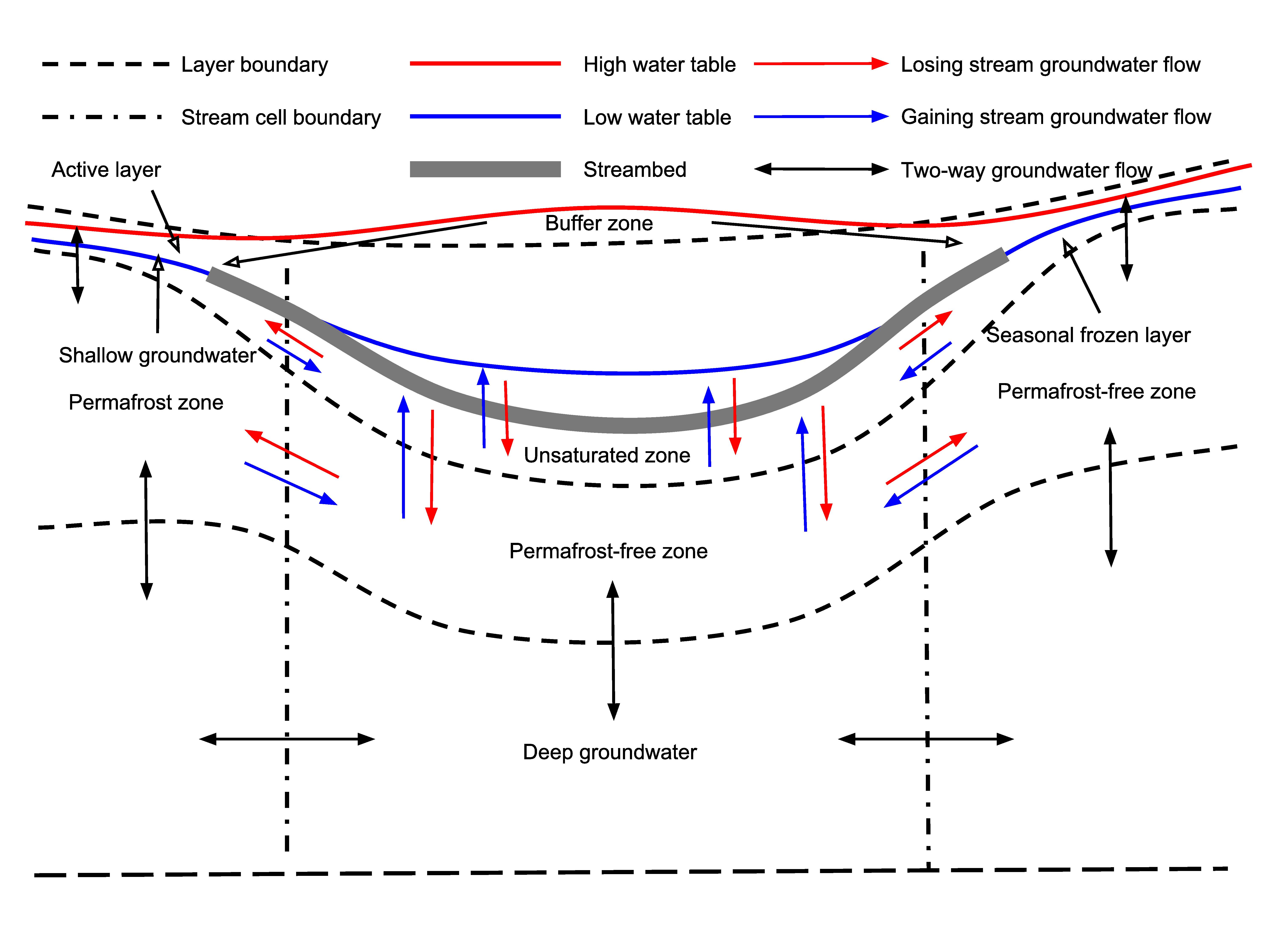
Figure 5. Interactions between a stream and a groundwater system underlain by permafrost and permafrost-free zones (not drawn to scale). The red (blue) line represents the high (low) gage height, and red (blue) arrows represent principal groundwater flow components when the stream is losing (gaining) water to (from) the groundwater system. The unsaturated zone may form beneath the streambed when a losing stream recharges the groundwater system. A large stream in the discontinuous-permafrost zone usually produces a temperature anomaly that forms a thaw bulb. The buffer zones were created to account for the lateral water flow between the stream channels and its banks (Liao and Zhuang, 2017).
Aquatic Biogeochemistry Model of CO2 and CH4
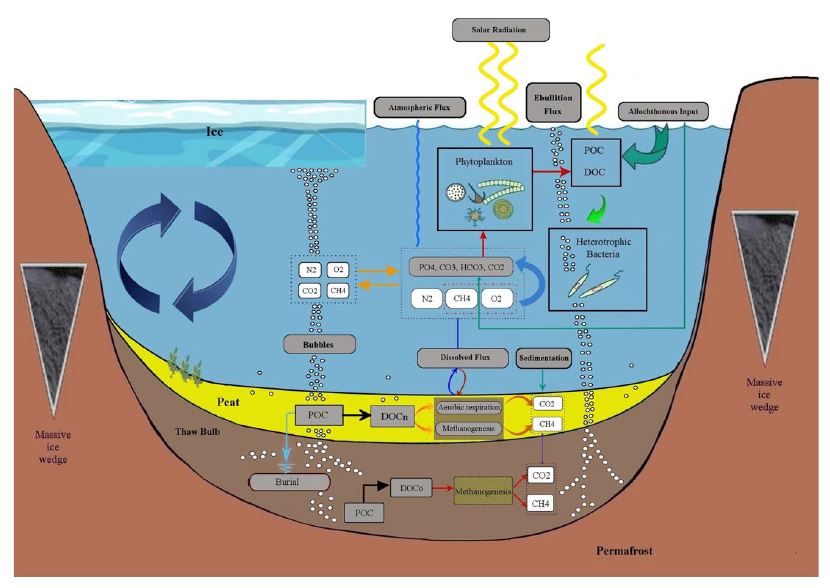
Figure 1. Simplified schematic of carbon and nutrient dynamics in the ALBM.
Global Soil CO Dynamics Model
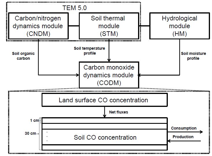
Figure 1. The model framework includes a carbon and nitrogen dynamics module (CNDM), a soil thermal module (STM) from Terrestrial Ecosystem Model (TEM) 5.0 (Zhuang et al., 2001, 2003), a hydrological module (HM) based on a land surface module (Bonan, 1996; Zhuang et al., 2004), and a carbon monoxide dynamics module (CODM). The detailed structure of CODM includes land surface CO concentration as the top boundary and 30 1 cm thick layers (in total, 30 cm) where consumption and production take place (Liu et al., 2018).
MIC-TEM
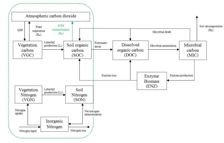
Schematic diagram of MIC-TEM. The green dashed circle is the previous structure used in TEM5.0 (Zhuang et al., 2003), without considering the effects of detailed microbial dynamics. The previous heterotrophic respiration is proportional to SOC (green dashed arrow). In MIC-TEM, new heterotrophic respiration considers the effects of microbial dynamics and enzyme kinetics. In addition, three new carbon pools (DOC, MIC, and ENZ) and five carbon fluxes (decomposition of SOC, microbial assimilation and death, enzyme production and loss) are considered (Zha and Zhuang 2018).
N2O-TEM
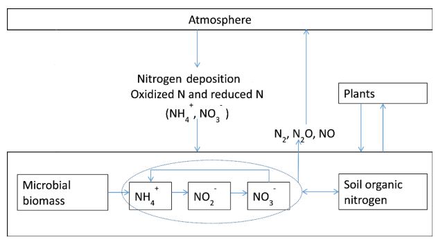
Schematic diagram of N2O emissions and N cycling between plants, soils, and the atmosphere: the input of N from the atmosphere to soils through nitrogen deposition as nitrate and ammonia, as well as microbial biomass dynamics, were modeled. Nitrification is modeled as a function of microbial biomass, soil organic nitrogen, and physical conditions; for more details refer to Yu (2016). N uptake by plants is modeled in the original TEM (McGuire et al., 1992).
XPTEM-XHAM
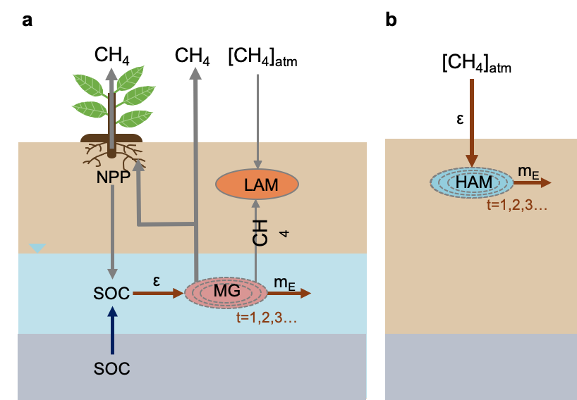
Fig. 1 | A schematic diagram of XPTEM-XHAM. a,b, The model simulates CH4 production by MGs and oxidation of CH4 by LAMs in wetlands (a) as well as the oxidation of [CH4]atm by HAMs in uplands (b). We used static inundation data33 to divide the Arctic landscape into wetland and upland regions but later varied the regions on the basis of time-varying inundation data34,35. Changes in MICbiomass of MGs and HAMs (grey dashed lines) depend on ε and mE, and are tracked as a function of time (t (h)). PSOC dynamics are added to account for SOC that is accessible from thawing permafrost when soil temperatures at the corresponding depths become higher than 1 °C. The dark blue arrow refers to PSOC dynamics, dark red arrows refer to microbial dynamics and grey arrows refer to processes from the original TEM. (Oh et al., 2020)
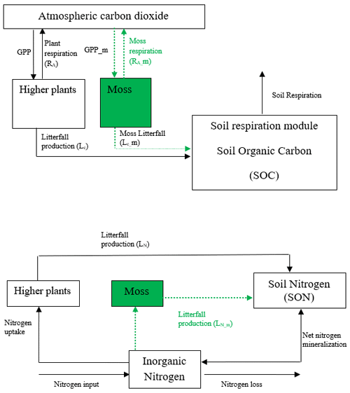
Fig. 2 Schematic diagram of TEM_Moss: green dashed arrows are new carbon and nitrogen fluxes, representing moss production, moss respiration, and litterfall of moss (Zha and Zhuang et al., 2021).
PTEM
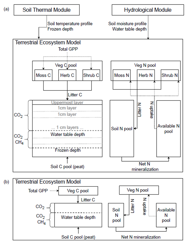
Figure. The structure of (a) the revised PTEM; and (b) the original Terrestrial Ecosystem Model (Zhao et al., 2022).
isoTEM
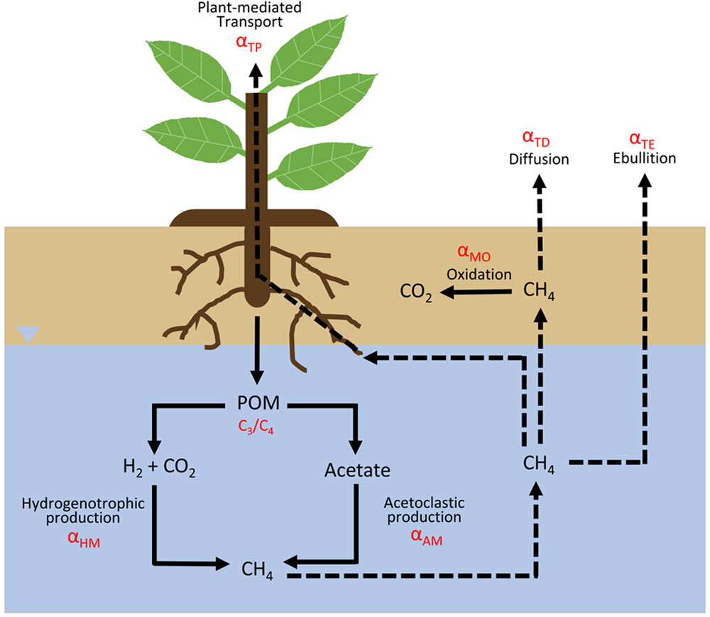
Figure. Schematic diagram of wetland CH4 dynamics and fractionations for isoTEM. (Oh et al., 2022).
A 3D ecosystem model ECO3D
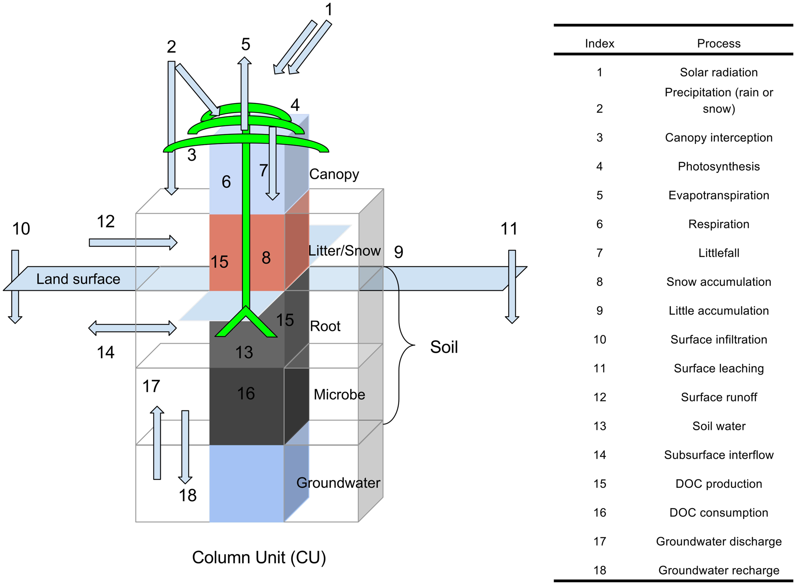
Figure. Water and carbon cycle processes simulated by the ECO3D model for a land column unit. Green lines and curves represent the vegetation. Blue arrows with indices represent key carbon and hydrological processes listed in the rightside table. The ECO3D model was developed based on a spatially distributed hydrological model, Precipitation Runoff Modeling System (PRMS) (Leavesley et al., 1983), and a process‐based biogeochemistry model, Terrestrial Ecosystem Model (TEM) (Zhuang et al., 2003). (Liao et al., 2019).
https://github.com/changliao1025/eco3d
The N Cycle in PTEM 2.3
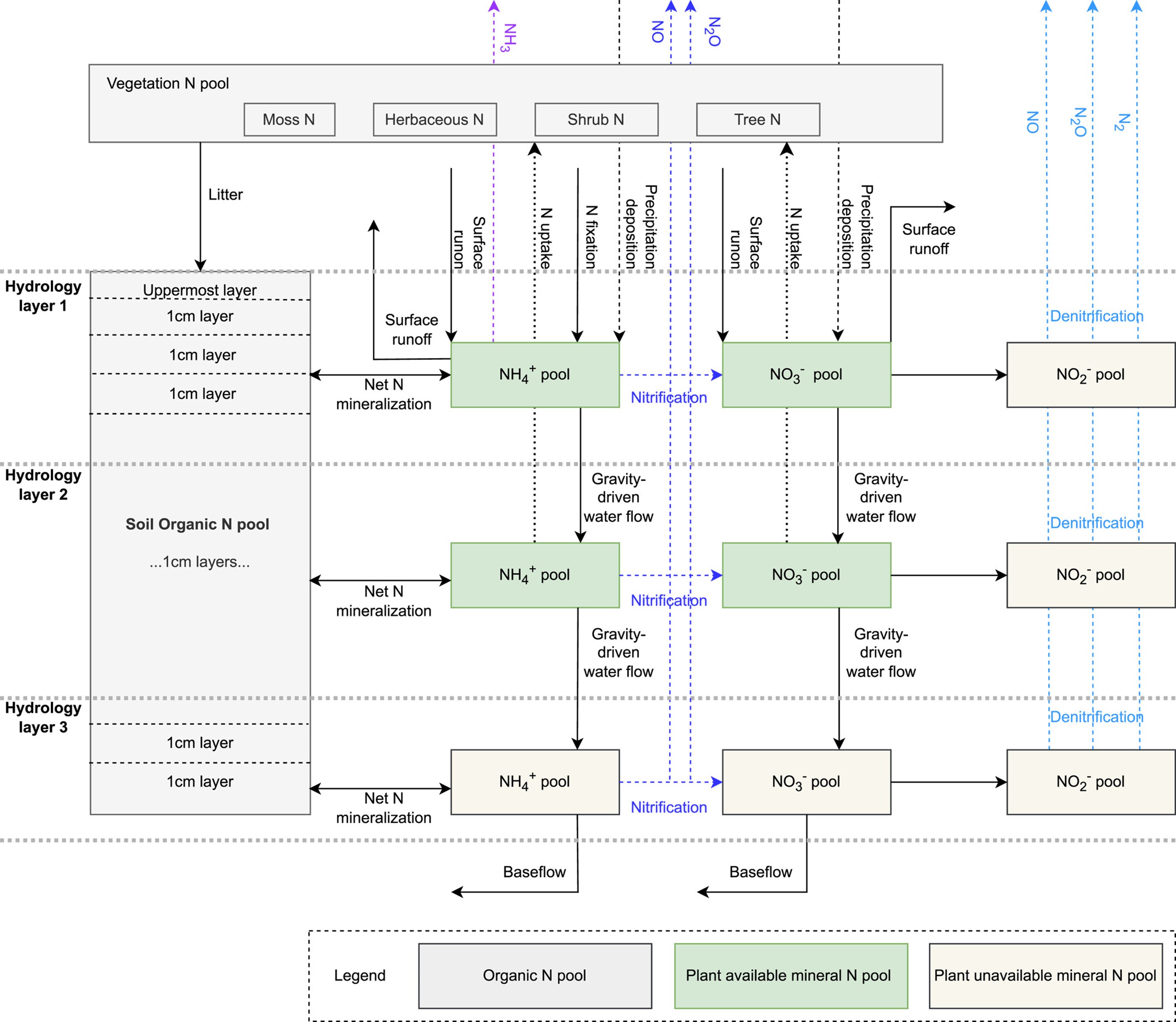
Figure. Nitrogen Cycling Feedback on Carbon Dynamics Leads to Greater CH4 Emissions and Weaker Cooling Effect of Northern Peatlands (Zhao, B. & Zhuang, Q. 2024).
N2O-TEM
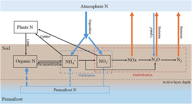
Nitrogen cycle and N2O production in the revised Terrestrial Ecosystem Model. Blue arrows represent nitrogen (N) inputs, while orange arrows represent nitrogen outputs. The active layer depth varies over time. Net mineralization: The difference between mineralization (organic N mineralized to inorganic N) and immobilization (inorganic N to organic N); Litter: organic N from plant litters; Uptake1: inorganic N uptake by plants; Deposition: atmospheric deposition of N; Emission: N2O emissions from soils; Uptake2: Atmospheric N2O uptake in soils (Yuan et al., 2025).
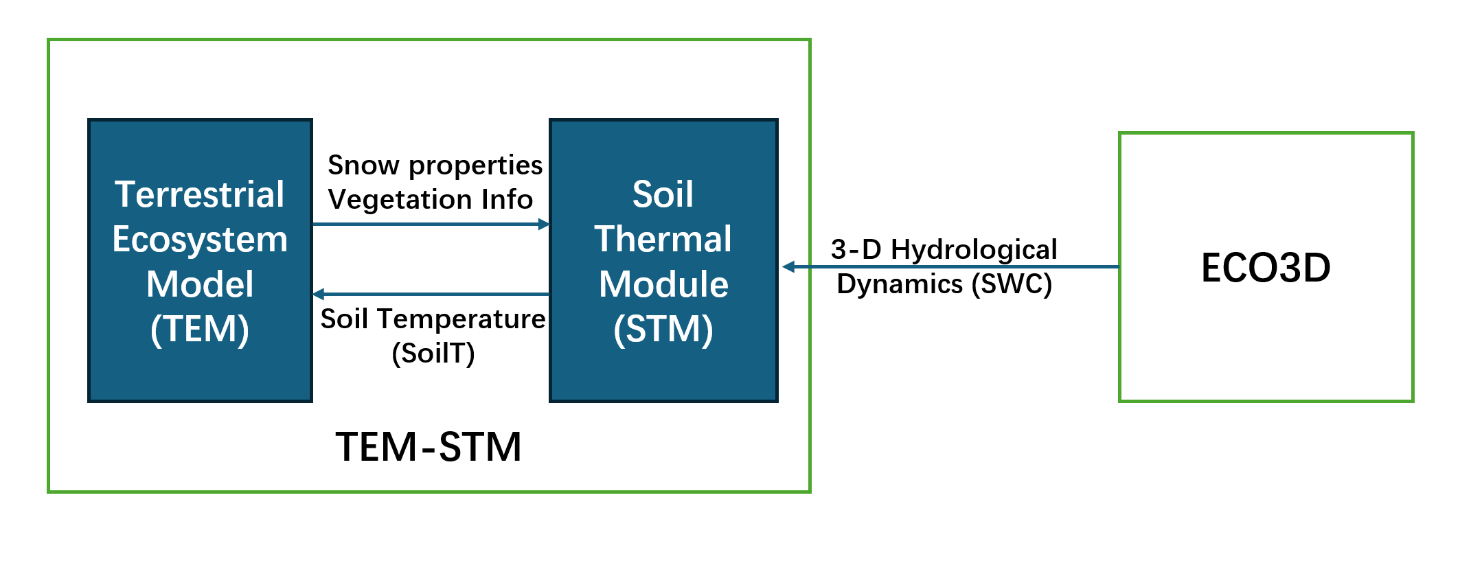
Structure of ECO3D-TEM-STM coupling (Liu et al., 2025)
N Fixation modeling in TEM:
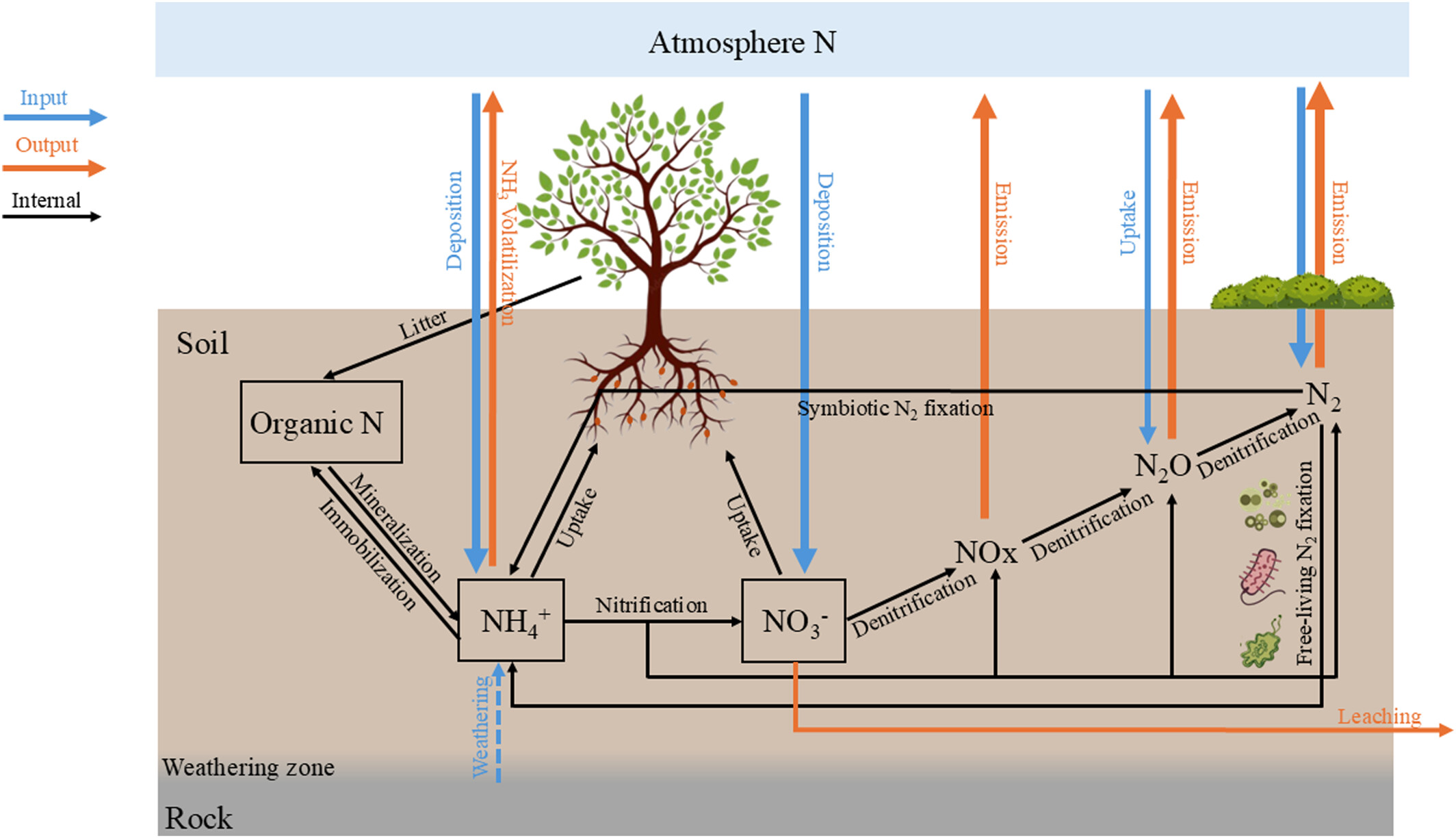
Nitrogen cycle and N2 fixation pathways in the revised terrestrial ecosystem model. Blue arrows represent nitrogen (N) inputs, while orange arrows represent nitrogen outputs. Mineralization: organic N mineralized to inorganic N; immobilization: inorganic N to organic N; litter: organic N from plant litters; Uptake (black): inorganic N uptake by plants; Deposition: atmospheric deposition of N; Emission: N2O emissions from soils; Uptake (blue): Atmospheric N2O uptake in soils; Symbiotic N2 fixation: N2 fixation through root nodules; Free-living nitrogen fixation: N2 fixation through soil microorganisms and moss, lichens and bryophytes (Yuan et al., 2025).

Structure of the nitrogen (N) cycle in Terrestrial Ecosystem Model (TEM), including three main components: external N inputs, internal cycling, and N outputs. Blue arrows indicate N input pathways, including atmospheric deposition, nitrogen release from rock weathering, biological nitrogen fixation, and atmospheric gas uptake. Orange arrows represent N output pathways, including leaching and gaseous losses (e.g., NH3, NOx, N2O, and N2). Black arrows illustrate internal nitrogen cycling within TEM, including litterfall, mineralization, immobilization, plant uptake, nitrification, and denitrification. Nitrogen leaching is represented primarily as nitrate loss because NO3− is highly mobile in soil water. Immobilization is represented mainly as microbial uptake of NH4+, reflecting the lower energetic cost of ammonium assimilation compared with nitrate reduction. (Yuan & Zhuang, 2026)