Mathematical and Statistical Techniques of Model and Data Assimilation
Conceptual diagram of the physics‐guided deep learning (PGDL) model framework and comparison with the PB model
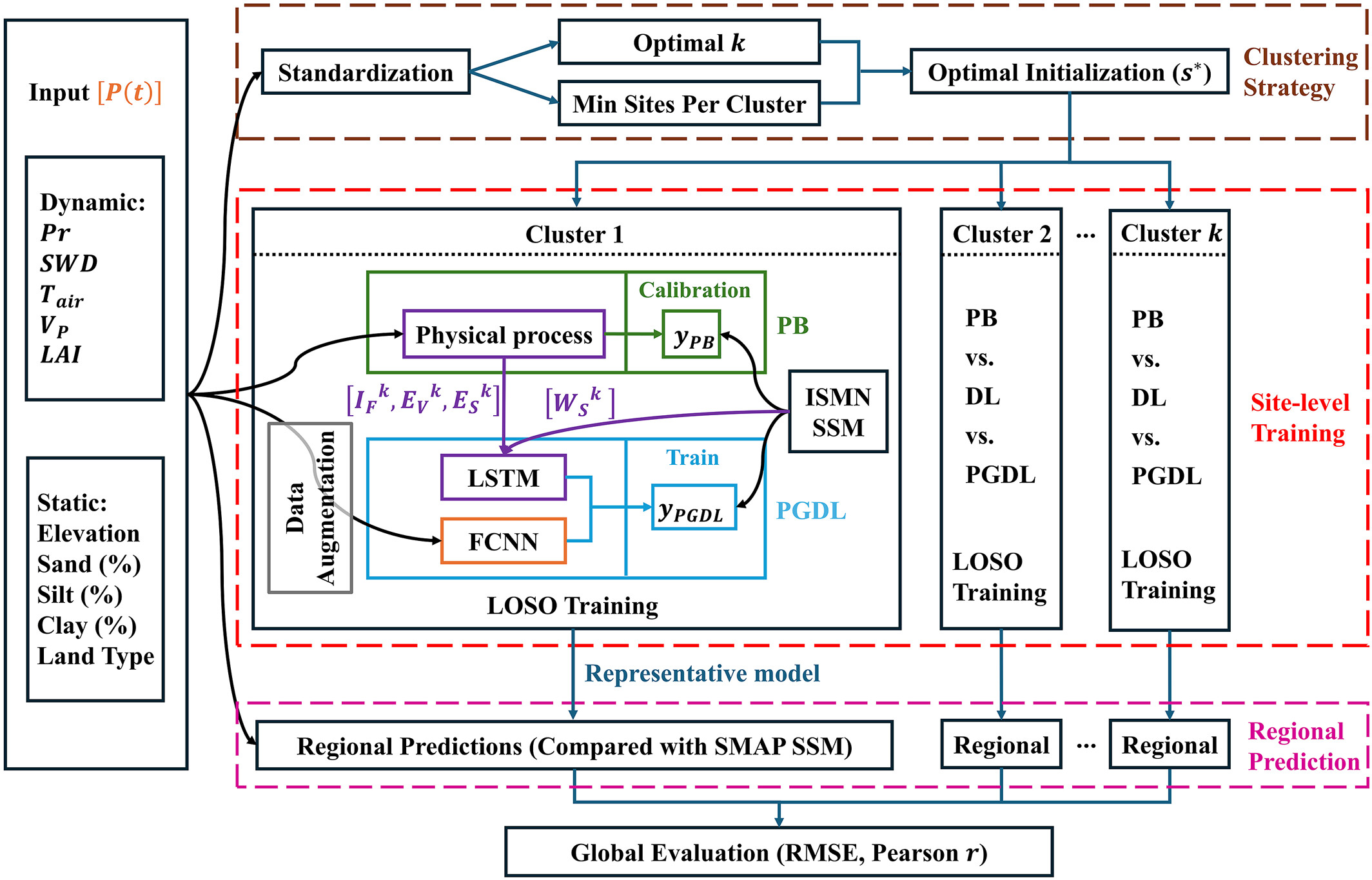
Workflow of the proposed methodology for global SSM prediction and evaluation. The framework integrates multi-source inputs, clustering-based regionalization, and comparative analysis across PB, DL, and PGDL models. Ten input features are first standardized and employed to derive the optimal clustering structure, defined by the number of clusters ( ) and a minimum number of sites per cluster, with the initialization subsequently selected based on the Silhouette Score. Within each cluster, DL and PGDL models are trained and evaluated in a cluster-specific manner, with a data augmentation step applied prior to site-level training when multiple ISMN sites share identical inputs within the same grid cell. The schematic of Cluster 1 presents the PGDL model architecture and its linkages to the PB model. The green section displays the PB process flow, and the blue section corresponds to the PGDL process. The purple box denotes the physical process represented in the PB model, with solid purple lines showing the coupling to the PGDL model through the transfer of
  ,
,  , and
, and  from PB outputs and
  from observations into the LSTM branch. The orange box represents the FCNN module processing the external inputs
  in the PGDL model. Both PB and PGDL models generate outputs (
 and
and  ) with their respective parameterization, and these outputs are evaluated against ISMN SSM observations through their respective calibration or training procedures. For each cluster, model performance is assessed under a LOSO scheme, and the best-performing model is selected as the representative model for regional prediction and validated against SMAP SSM. Finally, results across all clusters are aggregated to obtain a global evaluation. (Xi & Zhuang, 2026)
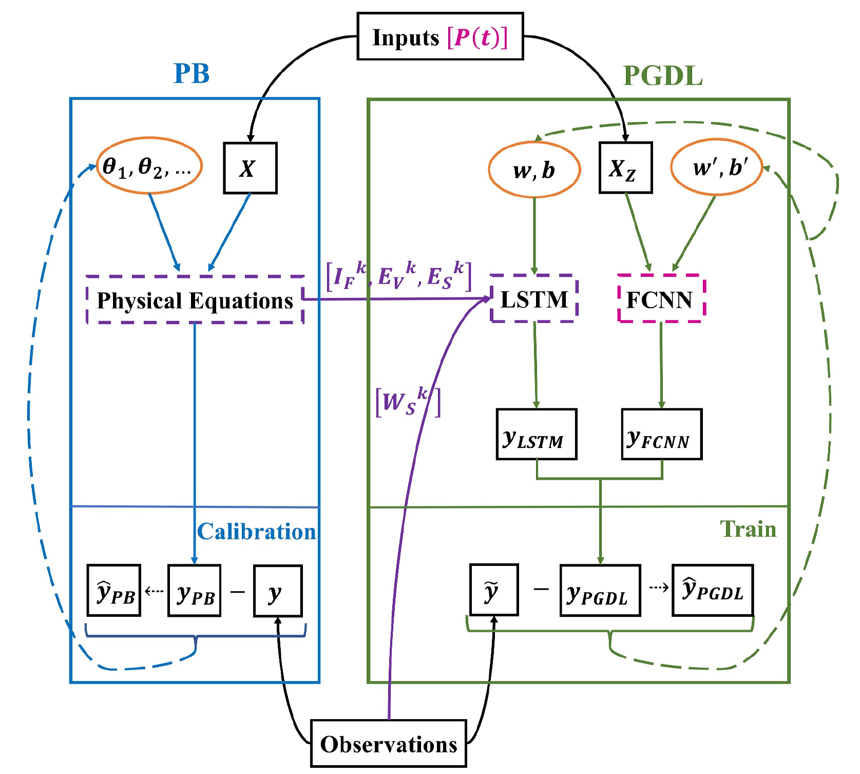
The blue part represents the workflow of the PB model, and the green part represents the workflow of the PGDL model. For the arrow lines, the solid lines represent the transfer of data, and the dotted lines represent the update of parameters. For the shapes, the black boxes represent data, the orange ellipses represent parameters, and the dashed boxes represent functional modules. The purple dashed box denotes the physical equation module in the PB model and its coupling with the PGDL model via the purple solid lines, which represent the flow of IF k, EV k, and ES k derived from the PB model and WS k from observations as inputs to the long short‐term memory (LSTM) branch. The pink dashed box represents the fully connected neural network (FCNN) module in the PGDL model, which processes the inputs P(t) . This structure highlights the input components in Equation 9 and their corresponding pathways in the model. Both PB and PGDL models receive input (X), consisting of both static and dynamic features, and then obtain the predictions (yPB and yPGDL) through calculation with corresponding parameters. Finally, the parameters are updated to obtain the optimized values ( ˆyPB and ˆyPGDL) by comparing with observations (y). θ∼ represents the parameters for the PB model. w and b denote the weight and bias parameters for the LSTM branch, and wʹ and bʹ denote the weight and bias parameters for the FCNN branch within the PGDL modeling framework. The differences between the two models are: (1) the PB model directly receives X, whereas the FCNN branch of the PGDL model receives normalized X (XZ); (2) the PB model directly uses y, whereas the PGDL model uses Kalman filtered y (˜y ). (Xi et al., 2025).
Global sensitivity analysis and Bayesian inference framework
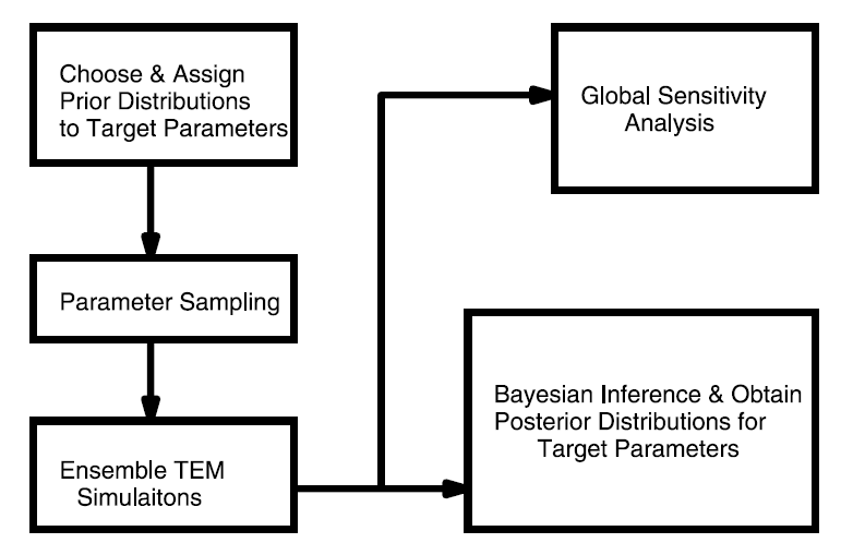
Our framework was based on Bayes' theorem: Pr(θ|V) Pr(V|θ) Pr(θ) where Pr(θ|V) is the posterior after Bayesian inference conditioned on available observations V (hereafter the bold letter indicates a matrix). θis the matrix of parameters and TEM outputs (e.g., GPP) and V is the matrix of observation or the matrix of the differences between prior simulations and the corresponding observations, whose element Vij denotes the type j data V(·)j at time step i. Pr(V|θ) is the likelihood function, which will be calculated as a function of TEM Monte Carlo simulations and the available eddy flux data. Pr(θ) is the prior of the TEM parameters and our estimated C fluxes (e.g., GPP, RESP and NEP) and EET. To address our research questions, we first conducted TEMensemble simulations with parameter priors. Second, the likelihood function Pr(V|θ) was calculated based on model simulations and observations. Third, the global sensitivity analysis was applied, and fourth, the Bayesian inference was conducted.
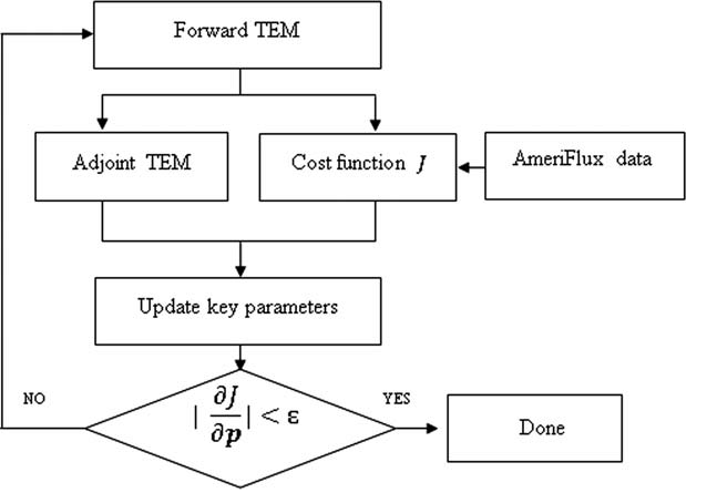
Adjoint code for a model could be either automatically generated using existing software, or generated manually, i.e., line-by-line. For example, the Tangent-linear and Adjoint Model Compiler (TAMC) [Giering and Kaminski, 1998], a software tool for generating first-order derivatives of models written in FORTRAN, has been widely used for atmospheric [Henze et al., 2007] and oceanic modeling [Marotzke et al., 1999; Stammer et al., 2002]. Here we manually developed the adjoint code directly from TEM model codes (where model ordinary differential equations have been discretized) with an attempt to better handle the processes in the model. The method was developed and applied for regional carbon studies (Zhu and Zhuang, 2013, 2014).